Day 5 — Basic Python
UBDS 2026: Basic Python
Day 5: Machine learning and data science
Topics covered / Сьогоднішні теми
- Basic exploratory data analysis (EDA) / Першопочаткове дослідження даних
- Correlation / Кореляція
- t-test / Тест Стьюдента
- One-way ANOVA / Дисперсійний аналіз
- Simple linear regression / Лінійна регресія
- microProject/RF / Мікропроект/метод випадкового лісу
We will use the palmers penguins dataset (palmerpenguins_extended.csv) which contains characteristics of penguins population over the years: Будемо використовувати набір даних про пінгвінів Палмера(palmerpenguins_extended.csv), що містить характеристики популяції цих пінгвінів впродовж кількох років:
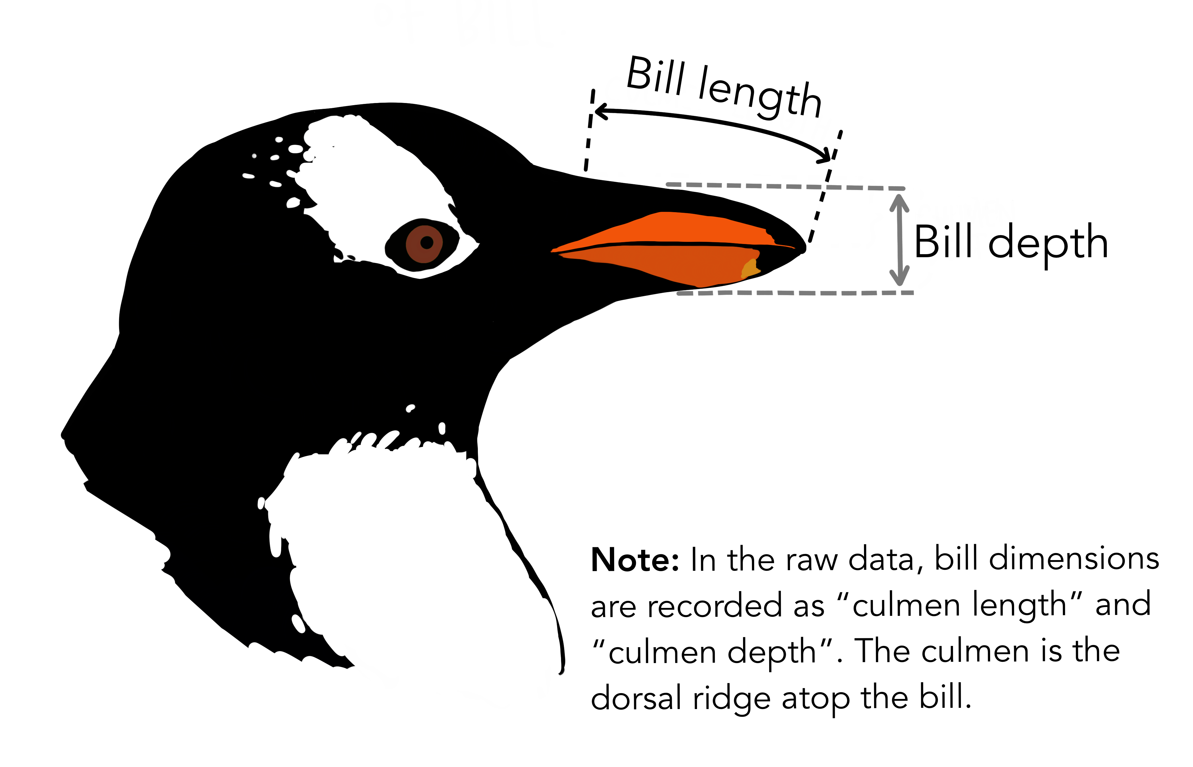
species/видisland/острівbill_length_mm/довжина клювуbill_depth_mm/глибина клювуflipper_length_mmдовжина плавцівbody_mass_g/маса тілаsex/статьdiet/дєтаlife_stage/стадія життяhealth_metrics/здоров'яyear/рік
Import the tools we need
pandashelps us work with tables of data / для роботи з таблицямиnumpyis needed to work with numerical data / для роботи з числовими даннимиmatplotlibhelps us make plots / для графіківscipy.statsgives us statistical tests / для статистичних тестівstatsmodelsgives us additional statistical tests / для додаткових тестівLinearRegressionfromsklearnhelps us build a simple regression model / для лінійної регресіїPolynomialFeaturesfrom sklearn gives us way to build polynomial models
import pandas as pd
import numpy as np
import matplotlib.pyplot as plt
from scipy import stats
from scipy.stats import shapiro
from statsmodels.stats.multicomp import pairwise_tukeyhsd
from sklearn.linear_model import LinearRegression
from sklearn.model_selection import train_test_split,cross_val_score
from sklearn.preprocessing import PolynomialFeatures, StandardScaler
Load the dataset
Note - be sure that file actually exist at the given location / Переконайтеся що вказаний шлях є вірним
Common name for a dataframe - df. / Типове ім’я для датафрейму ДФ.
df = pd.read_csv("palmerpenguins_extended.csv")
df
First look at the data
To repeat previous lesson - please print: / Для закріплення вчорашнього дня - будь ласка визначте - the first few rows / Перші кілька строчок
- the last few rows / Останні кілька строчок - the shape of the table / Форма таблиці - the column names / Імена колонок - the data types in each column / Типи даних в колонках - rows number 5 and 10 / строчки номер 5 і 10 - flipper length column / колонку що містить довжину плавців
# Your code goes here# Your code goes here# Your code goes here# Your code goes here# Your code goes here# Your code goes here# Your code goes hereMissing values
A missing value is called NA(NA-Not assesed) and it means some information is absent / Відсутнє значення називають NA, і це значить що частина інформації відсутня.
We can count missing values in each column like this / Ми можемо порахувати відсутні значення наступним чином.
df.isna().sum()We have two strategies how to deal with NA. First one is simply removing them. / У нас є дві стратегії як розбиратися з NA. Перший варіант просто їх прибрати.
df_drop = df.dropna()
df_drop.shapedf_drop.isna().sum()Second option is to impute them using mean or median / Наступний варіант це заповнити їх використовуючи середнє чи медіану
df_fill = df.copy()

df_fill["body_mass_g"] = df_fill["body_mass_g"].fillna(
    df_fill["body_mass_g"].mean()
)

df_fill["flipper_length_mm"] = df_fill["flipper_length_mm"].fillna(
    df_fill["flipper_length_mm"].median()
)

#inpute lenght of bil with mean and depth of bill with median / зааповніть довжину клюва середнім значенням і глибину клюва медіаною

#

df_fill.isna().sum()df=df.dropna()Looking at categories
Some columns contain categories, not numbers. / В деяких колонках маємо категорії а не числа
Examples: - species - island - sex - diet - life_stage - health_metrics
df["species"].unique()df["island"].unique()df["sex"].unique()df["life_stage"].unique()df["health_metrics"].unique()Exercise 2
Use the .unique() results above to answer:
- How many species are in the dataset?
- How many islands are in the dataset?
Basic descriptive statistics
Descriptive statistics help us summarize numeric variables. / Описова статистика допомогає нам дослідити числові значення.
Typical examples: - mean - standard deviation - minimum - maximum - quartiles
We can get using one function / Для цього у нас є одна проста функція
df.describe()Focus on one variable
We can also inspect one column at a time. / Також ми можемо отримати таку статистику для однієї колонки
df["body_mass_g"].describe()Simple filtering
Filtering means selecting only the rows we want / Фільтрування обирає тільки ті строчки що відповідають певній умові
For repetition filter: - only Adelie penguins - only adult penguins - only male penguins - only penguins from Biscoe island and male:
# Your code goes here# Your code goes here# Your code goes here# Your code goes hereCounting categories
To work with categories we can count them. / Аби працювати з категоріями ми можемо їх порахувати
For that we use value_counts().
df["species"].value_counts()Exercise: write your answer in this editable Python cell.
Relative frequencies
Sometimes we want percentages instead of raw counts. / Інколи ми хочемо оперувати не сирими значеннями, а частотами
We can do that with normalize=True.
df["species"].value_counts(normalize=True)Group summaries
Group summaries are used to count group-wise statistics. / Групування використовується аби рахувати погрупову статистику.
As a reminder lets calculate / Як нагадування давайте порахуємо - What is the average body mass for each species? / Середю вагу для різних видів - What is the avrage flipper length for each island? / Середню довжину плавців на різних островах - What is the median bill length for males and females? / Медіанну довжини клюва серед різних статей - What is the frequencies of different species occurence on each island/ Якою є частота різних видів на кожному острові
The general pattern is: df.groupby("group_column")["numeric_column"].mean()
df.groupby("species")["body_mass_g"].mean()# Your code goes here# Your code goes here# Your code goes hereGroup by more than one column
We can also group by two variables. Також можна групувати по двом або більше колонкам
df.groupby(["species", "sex"])["body_mass_g"].mean()Histogram
A histogram shows the distribution of one numeric variable.
Here we plot body_mass_g.
plt.figure(figsize=(8, 5))
plt.hist(df["body_mass_g"], bins=20)
plt.title("Distribution of body mass")
plt.xlabel("Body mass (g)")
plt.ylabel("Count")
plt.show()
Bar chart of category counts
Bar charts are useful for categorical variables.
Here we count penguins by species.
species_counts = df["species"].value_counts()

plt.figure(figsize=(8, 5))
plt.bar(species_counts.index, species_counts.values)
plt.title("Number of penguins by species")
plt.xlabel("Species")
plt.ylabel("Count")
plt.show()
Scatter plot
A scatter plot shows the relationship between two numeric variables.
Here we compare: - flipper_length_mm - body_mass_g
plt.figure(figsize=(8, 5))
plt.scatter(df["flipper_length_mm"], df["body_mass_g"])
plt.title("Body mass vs flipper length")
plt.xlabel("Flipper length (mm)")
plt.ylabel("Body mass (g)")
plt.show()
Boxplot
A boxplot helps compare distributions across groups.
Here we compare body mass for the three species.
adelie_mass = df[df["species"] == "Adelie"]["body_mass_g"]
chinstrap_mass = df[df["species"] == "Chinstrap"]["body_mass_g"]
gentoo_mass = df[df["species"] == "Gentoo"]["body_mass_g"]

plt.figure(figsize=(8, 5))
data_box=[adelie_mass, chinstrap_mass, gentoo_mass]
plt.boxplot(data_box, labels=["Adelie", "Chinstrap", "Gentoo"])
plt.title("Pengui")
plt.ylabel("Body mass")
plt.show()
Make the following plots:
- histogram of
bill_length_mm - bar chart of counts for
life_stage - scatter plot of
bill_length_mmvsbill_depth_mm - boxplot of
flipper_length_mmby sex
# Your code goes here# Your code goes here# Your code goes here# Your code goes hereCorrelation
Corelation measure the strength and direction of a linear(and non-linear) relationship between two numeric variables. / Кореляція вимірює сили та напрямок лінійного та нелінійного зв’язку між двома змінними
The correlation coefficient is usually written as r.
Its values are between -1 and 1.
- close to
1strong positive relationship - close to
-1strong negative relationship - close to
0weak or no linear relationship
df["body_mass_g"].corr(df["flipper_length_mm"])How to work - with non-linear relationship - Spearman correlation(but first normality test) / Як працювати з нелінійною кореляцією - використовувати кореляцію Спірмана, перед тим перевіривши номральність
stat, p_value = shapiro(df["body_mass_g"])

print("Shapiro test statistic:", stat)
print("p-value:", p_value)
stat, p_value = shapiro(df["flipper_length_mm"])
print("Shapiro test statistic:", stat)
print("p-value:", p_value)If our pvalue <0.05 we can assume non-normality, in this case lets use Spearman correlation
num_df = df[["body_mass_g","bill_depth_mm"]].dropna()

corr_spearman = num_df.corr(method="spearman")

print("\nSpearman correlation:\n", corr_spearman)
Calculate Spearman and Pearson correlation for body mass and flippers lenght / Порахуйте кореляцію Спірмана та Пірсона для маси тіла та довжини плавців.
# Your code goes hereCorrelation matrix
A correlation matrix shows pairwise correlations for several numeric variables at once. We can make a table out of it.
numeric_cols = ["bill_length_mm", "bill_depth_mm", "flipper_length_mm", "body_mass_g", "year"]
df[numeric_cols].corr()
corr = df[numeric_cols].corr(method="spearman")
plt.figure(figsize=(6, 5))
plt.imshow(corr, interpolation='nearest')
plt.colorbar()
plt.xticks(range(len(corr.columns)), corr.columns, rotation=45)
plt.yticks(range(len(corr.columns)), corr.columns)
for i in range(len(corr.columns)):
for j in range(len(corr.columns)):
plt.text(j, i, f"{corr.iloc[i, j]:.2f}",
ha='center', va='center', color='black')
plt.title("Correlation Matrix (Pearson)")
plt.tight_layout()
plt.show()Not all python libraries are made equal - seaborn provide much faster and easier way to do same plot
import seaborn as sns
num_df = df[numeric_cols].apply(pd.to_numeric, errors="coerce")
corr = num_df.corr(method="spearman")


sns.heatmap(
    corr,
    annot=corr.values,
    cmap="coolwarm",
    center=0,
    square=True)

plt.title("Correlation Matrix (Seaborn)")
plt.xticks(rotation=45)
plt.tight_layout()
plt.show()corr.valuest-test
A t-test compares the means of two groups. / Т-тест потрібен для порівняння двох груп.
We need: - one numeric variable - one grouping variable with two groups
Do adult male and adult female penguins differ in average body mass? / Чи мають дорослі самці і самки відмінності у масі тіла?
adult = df[df["life_stage"] == "adult"]

male_mass = adult[adult["sex"] == "male"]["body_mass_g"]
female_mass = adult[adult["sex"] == "female"]["body_mass_g"]

male_mass.describe(), female_mass.describe()
Hypotheses of the t-test
- Null hypothesis (H0): the mean body mass is the same in adult males and adult females
- Alternative hypothesis (H1): the mean body mass is different
We will use Welch’s t-test by setting equal_var=False.
ttest_result = stats.ttest_ind(male_mass, female_mass, equal_var=False)
ttest_result
Interpreting the result
The output gives: - a t statistic - a p-value
If the p-value is small, we reject the null hypothesis.
A common threshold is 0.05.
- if
p < 0.05: evidence of a difference - if
p >= 0.05: not enough evidence of a difference
Run a t-test to compare bill_length_mm between male and female adult penguins.
Steps: 1. filter only adults 2. split bill length into male and female groups 3. run stats.ttest_ind 4. compare the means
# Your code goes heremale_bill.mean(), female_bill.mean()One-way ANOVA
ANOVA stands for Analysis of Variance. It is needed to compare more than 2 groups.
Do adult penguin species differ in average flipper length?
adult = df[df["life_stage"] == "adult"]

adelie_flipper = adult[adult["species"] == "Adelie"]["flipper_length_mm"]
chinstrap_flipper = adult[adult["species"] == "Chinstrap"]["flipper_length_mm"]
gentoo_flipper = adult[adult["species"] == "Gentoo"]["flipper_length_mm"]

adult.groupby("species")["flipper_length_mm"].mean()
anova_result = stats.f_oneway(adelie_flipper, chinstrap_flipper, gentoo_flipper)
anova_resultHypotheses for ANOVA
- Null hypothesis (H0): all group means are equal
- Alternative hypothesis (H1): at least one group mean is different
If the p-value is below 0.05, we conclude that not all means are equal.
Important ANOVA note
ANOVA tells us that a difference exists somewhere among the groups. / Анова каже нам чи існує різниця між групами It does not automatically tell us exactly which pairs differ. / Вона не каже, між якими саме групами To get whihc groups differs we need to run post-hoc test - TukeyHSD. / Щоб це визначити маємо використати додатковий тест-Тьюкі
anova_data = df[["species", "flipper_length_mm"]].dropna()

tukey = pairwise_tukeyhsd(
    endog=anova_data["flipper_length_mm"],
    groups=anova_data["species"],
    alpha=0.05)

print(tukey)
Use one-way ANOVA to test whether mean body mass differs among the three species.
Steps: 1. filter to adults / Відфільтруйте дорослих 2. create three groups / Створіть три групи 3. run stats.f_oneway / Проведіть анову 4. run post hoc test / Проведіть тест тьюкі
# Your code goes hereSimple linear regression
Linear regression models the relationship between: / Лінійна регресія визначає зв’язок між одним предиктором(Х-змінна) та одним цільовим значенням (У-змінна)
- one predictor variable
X - one or more outcome variable
y
We will predict:
body_mass_gfromflipper_length_mm
This is called simple linear regression because there is only one predictor.
Exercise: write your answer in this editable Python cell.
The general idea
The model tries to find a line:
predicted body mass = intercept + slope × flipper length
- the intercept is where the line starts
- the slope tells us how much the predicted outcome changes when the predictor increases by 1 unit
X = df[["flipper_length_mm"]]
y = df["body_mass_g"]

model = LinearRegression()
model.fit(X, y)
Model coefficients
model.coef_, model.intercept_Interpretation
If the slope is positive, then larger flipper length is associated with larger predicted body mass.
R-squared
R^2 tells us how much variation in the outcome is explained by the predictor.
- closer to 1 means stronger explanatory power
- closer to 0 means weaker explanatory power
model.score(X, y)Make predictions
We can ask the model to predict body mass for given flipper lengths.
new_penguins = pd.DataFrame({"flipper_length_mm": [180, 190, 200, 210, 220]})
model.predict(new_penguins)
Plot the regression line
We will: 1. draw the scatter plot 2. create predicted values 3. draw a line through those predictions
predicted_y = model.predict(X)

plt.figure(figsize=(8, 5))
plt.scatter(X["flipper_length_mm"], y)
plt.plot(X["flipper_length_mm"], predicted_y, color="red")
plt.title("Linear regression: body mass vs flipper length")
plt.xlabel("Flipper length")
plt.ylabel("Body mass")
plt.show()
Fit a linear regression model to predict bill_depth_mm from body_mass_g.
Tasks: 1. create X from bill_length_mm 2. create y from body_mass_g 3. fit a LinearRegression() model 4. print the slope, intercept, and R^2
# Your code goes hereLinear regression can include more than 1 variable, it is called Multiple Linear Regression
General formula would look like predicted body mass = intercept + slope1 × flipper length + slope2 × bill length + slope3 × bill depth
X = df[["bill_length_mm", "bill_depth_mm", "flipper_length_mm"]]
y = df["body_mass_g"]

model = LinearRegression()
model.fit(X, y)

print("Intercept:", model.intercept_)
print("Coefficients:", model.coef_)
model.score(X, y)Feature scaling (normalization)
In regression, different features may have very different scales:
- body_mass_g in thousands units - g
- bill_length_mm in tens units - mm
This can affect: - interpretation of coefficients - numerical stability of models
Two common approaches:
Standardization (Z-score)
transforms data to mean = 0, std = 1Min-Max scaling
scales data between 0 and 1
df[["bill_length_mm","flipper_length_mm","body_mass_g"]].dropna().describe()data_sc= df[[
"bill_length_mm",
"bill_depth_mm",
"flipper_length_mm",
"body_mass_g"]].dropna()
X = data_sc.drop(columns=["body_mass_g"])
y = data_sc["body_mass_g"]
scaler = StandardScaler()
X_scaled = scaler.fit_transform(X)
X_scaled = pd.DataFrame(X_scaled, columns=X.columns)
X_scaled.head()model_scaled = LinearRegression()
model_scaled.fit(X_scaled, y)
print("R²:", model_scaled.score(X_scaled, y))print("Original coefficients:")
for name, coef in zip(X.columns, model.coef_):
print(f"{name}: {coef:.2f}")
print("Scaled coefficients:")
for name, coef in zip(X.columns, model_scaled.coef_):
print(f"{name}: {coef:.2f}")Regression can include not only numerical, but also a categorical features To add them to our model they must be converted into numerical form.
One common method is one-hot encoding: - each category becomes a separate column - values are 0 or 1
data = df[["bill_length_mm", "bill_depth_mm", "flipper_length_mm", "species", "body_mass_g"]]

data_encoded = pd.get_dummies(data,  columns=["species"], drop_first=True)
data_encoded
X = data_encoded.drop(columns=["body_mass_g"])
y = data_encoded["body_mass_g"]
model = LinearRegression()
model.fit(X, y)
print("Intercept:", model.intercept_)
for name, coef in zip(X.columns, model.coef_):
print(f"{name}: {coef:.2f}")model.score(X, y)Why there cannot be one general solution
Sometimes one regression line is not enough for the whole dataset.
If the dataset contains groups, such as islands, each group may have a different relationship between variables.
Here we will build a separate regression for each island and plot them together.
reg_data = df[["island", "flipper_length_mm", "body_mass_g"]].dropna()


plt.figure(figsize=(8, 6))

for island in reg_data["island"].unique():
    island_data = reg_data[reg_data["island"] == island]

    X = island_data[["flipper_length_mm"]]
    y = island_data["body_mass_g"]

    model = LinearRegression()
    model.fit(X, y)

    y_pred = model.predict(X)
    sorted_idx = island_data["flipper_length_mm"].argsort()
    x_sorted = island_data["flipper_length_mm"].iloc[sorted_idx]
    y_sorted = y_pred[sorted_idx]

    plt.scatter(
        island_data["flipper_length_mm"],
        island_data["body_mass_g"],
        alpha=0.6,
        label=f"{island} data")

    plt.plot(
        x_sorted,
        y_sorted,
        linewidth=2,
        label=f"{island} regression")

plt.xlabel("Flipper length")
plt.ylabel("Body mass")
plt.title("Separate regression lines for each island")
plt.legend()
plt.show()
Now lets create a tidy function from the messy code above
def plot_grouped_regression(data, group_col, x_col, y_col):
    plt.figure(figsize=(8, 6))

    for group in data[group_col].unique():
        group_data = data[data[group_col] == group]

        X = group_data[[x_col]]
        y = group_data[y_col]

        model = LinearRegression()
        model.fit(X, y)

        y_pred = model.predict(X)

        sorted_idx = group_data[x_col].argsort()
        x_sorted = group_data[x_col].iloc[sorted_idx]
        y_sorted = y_pred[sorted_idx]

        plt.scatter(group_data[x_col], group_data[y_col], alpha=0.6, label=f"{group} data")
        plt.plot(x_sorted, y_sorted, linewidth=2, label=f"{group} regression")

    plt.xlabel(x_col)
    plt.ylabel(y_col)
    plt.title(f"Separate regression lines for each {group_col}")
    plt.legend()
    plt.show()
island_data = df[["island", "flipper_length_mm", "body_mass_g"]]
plot_grouped_regression(island_data, "island", "flipper_length_mm", "body_mass_g")Now please build a separate regression line for each species/ Тепер побудуйте окрему модель лінійної регресії для кожного виду
# Your code goes hereTrain/Test Split
When building a model, we should not evaluate it on the same data we used for training. / Коли ми тренуємо нашу модель ми маємо визначати її точність не на тих самих даних на яких тренували(не так як ми робили вище;)
Instead, we split the dataset into:
- training set used to train the model
- test set used to evaluate the model
This helps us understand how well the model performs on new, unseen data.
X = data_encoded.drop(columns=["body_mass_g"])
y = data_encoded["body_mass_g"]


X_train, X_test, y_train, y_test = train_test_split(X, y, test_size=0.2,  random_state=2026)

print("Train shape:", X_train.shape)
print("Test shape:", X_test.shape)
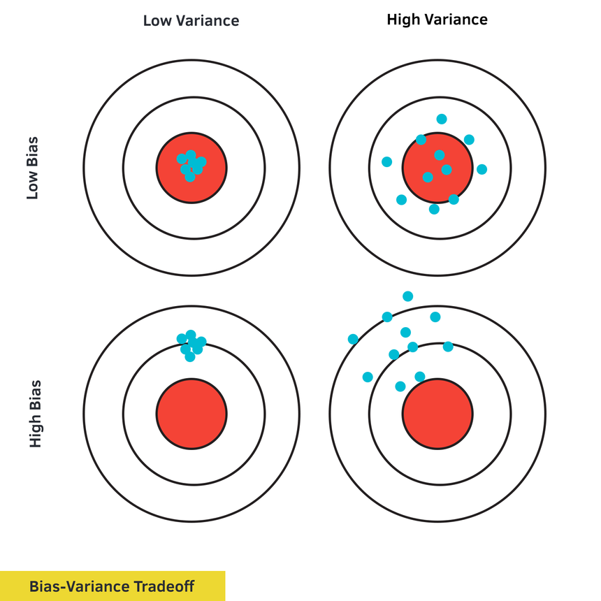
If Train R ≈ Test R model generalizes well
If Train R > Test R model may be overfitting
model = LinearRegression()
model.fit(X_train, y_train)

train_score = model.score(X_train, y_train)
test_score = model.score(X_test, y_test)

print("Train R:", train_score)
print("Test R:", test_score)
Cross-validation
Train/test split uses only one split of the data.
Cross-validation improves this by: splitting data multiple times training and testing multiple models averaging the results
This gives a more reliable estimate of model performance.
model = LinearRegression()
scores = cross_val_score(model, X,y, cv=5,  scoring="r2")

print("Cross-validation scores:", #Wat should be there ?/Якого аргументи не вистачає?)
#Also provide average score / Також порахуйте середню точність моделі
print("Mean R²:", #
Exercise: write your answer in this editable Python cell.
- Change test_size to 0.3. What happens? / Змініть розміри тест сету, як змінюютсья резульати?
- Try cv=3 and cv=10. How do results change? / Спробуйте використати іншу кількість валідацій. Як змінюються результати?
Exercise: write your answer in this editable Python cell.
Polynomial regression on synthetic data
In real datasets relationships are not always perfectly linear.
To understand polynomial regression clearly, we will first create some synthetic non-linear data
np.random.seed(2026)
x = np.linspace(0, 10, 80)
y = 3 + 2 * x + 2 * x**2 + np.random.normal(0, 8, size=len(x))


poly_df = pd.DataFrame({"x": x, "y": y})

poly_df.head()plt.figure(figsize=(6, 4))
plt.scatter(poly_df["x"], poly_df["y"])
plt.xlabel("x")
plt.ylabel("y")
plt.title("Synthetic non-linear data")
plt.show()X = poly_df[["x"]]
y = poly_df["y"]
linear_model = LinearRegression()
linear_model.fit(X, y)
print("Intercept:", linear_model.intercept_)
print("Coefficient:", linear_model.coef_[0])
print("R:", linear_model.score(X, y))y_pred_linear = linear_model.predict(X)
plt.figure(figsize=(6, 4))
plt.scatter(poly_df["x"], poly_df["y"], label="Data")
plt.plot(poly_df["x"], y_pred_linear, label="Linear regression")
plt.xlabel("x")
plt.ylabel("y")
plt.title("Linear regression on synth curved data")
plt.legend()
plt.show()poly = PolynomialFeatures(degree=2, include_bias=False)
X_poly = poly.fit_transform(X)
X_polypoly_model = LinearRegression()
poly_model.fit(X_poly, y)
print("Intercept:", poly_model.intercept_)
print("Coefficients:", poly_model.coef_)
print("R:", poly_model.score(X_poly, y))y_pred_poly = poly_model.predict(X_poly)
plt.figure(figsize=(6, 4))
plt.scatter(poly_df["x"], poly_df["y"], label="Data")
plt.plot(poly_df["x"], y_pred_poly, label="Polynomial regression")
plt.xlabel("x")
plt.ylabel("y")
plt.title("Polynomial regression on curved data")
plt.legend()
plt.show()plt.figure(figsize=(6, 4))
plt.scatter(poly_df["x"], poly_df["y"], label="Data")
plt.plot(poly_df["x"], y_pred_linear, label="Linear regression")
plt.plot(poly_df["x"], y_pred_poly, label="Polynomial regression")
plt.xlabel("x")
plt.ylabel("y")
plt.title("Linear vs Polynomial Regression")
plt.legend()
plt.show()Underfitting vs Overfitting
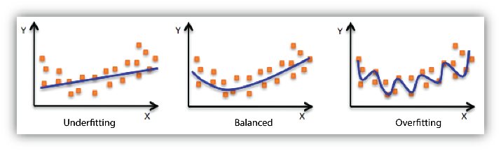
When training a model, there are two common problems:
Underfitting
- model is too simple
- cannot capture the pattern in the data
- poor performance on both training and test data
Overfitting
- model is too complex
- fits training data very well
- performs poorly on new (test) data
We will demonstrate this using polynomial regression.
degrees = [1, 2, 3, 4, 5, 6, 7, 8, 9, 10, 12, 15, 20]

results = []

for d in degrees:
    poly = PolynomialFeatures(degree=d, include_bias=False)

    X_train_poly = poly.fit_transform(X_train)
    X_test_poly = poly.transform(X_test)

    model = LinearRegression()
    model.fit(X_train_poly, y_train)

    train_r2 = model.score(X_train_poly, y_train)
    test_r2 = model.score(X_test_poly, y_test)

    results.append((d, train_r2, test_r2))

for d, train_r2, test_r2 in results:
    print(f"Degree {d}: Train R²={train_r2:.3f}, Test R²={test_r2:.3f}")
Interpretation
- Degree 1 underfitting (too simple)
- Degree 2 good balance
- Degree 10 verfitting (too complex)
Look at the difference between Train and Test R²: - small difference means good model - large difference means overft
Competition - we hid part of this dataset from you. Now we will provide it, but without bodymass column, and you will try to build a model yourself with the best possible R squared . Hints: - include additional features - exclude some features - try different poly transformations and their degrees - try preprocess your data - Get back to NA treatment - all of the above
Exercise: write your answer in this editable Python cell.